[ ]:
Data Interpolation and Imputation
This tutorial demonstrates data-wrangler’s capabilities for handling missing data through interpolation and imputation techniques. These are essential for cleaning real-world datasets.
Overview
Data-wrangler provides several approaches for handling missing data:
Interpolation: Fill missing values using mathematical interpolation methods
Model-based imputation: Use machine learning models to predict missing values
Statistical imputation: Fill with statistical measures (mean, median, mode)
Custom imputation: Define your own missing data handling strategies
Let’s explore these techniques with practical examples.
[1]:
import datawrangler as dw
import pandas as pd
import numpy as np
import matplotlib.pyplot as plt
from datawrangler.decorate import funnel, interpolate
Interpolation with @interpolate
The @interpolate decorator cleans missing values (NaN) out of the data before your function runs. You control it at call time with the interp_kwargs keyword. Passing interp_kwargs={'method': 'linear'} fills gaps by linear interpolation (any method supported by pandas.DataFrame.interpolate works).
[2]:
# Build a small signal and knock some values out
np.random.seed(0)
x = np.linspace(0, 4 * np.pi, 24)
signal = np.sin(x)

data = pd.DataFrame({'a': signal, 'b': np.cos(x), 'c': signal + np.random.randn(24) * 0.1})
data.loc[[3, 4, 5], 'a'] = np.nan
data.loc[[10, 11], 'b'] = np.nan
data.loc[[17], 'c'] = np.nan
print(f'Missing values before cleaning: {int(data.isna().sum().sum())}')
data.head(8)
Missing values before cleaning: 6
[2]:
| a | b | c | |
|---|---|---|---|
| 0 | 0.000000 | 1.000000 | 0.176405 |
| 1 | 0.519584 | 0.854419 | 0.559600 |
| 2 | 0.887885 | 0.460065 | 0.985759 |
| 3 | NaN | -0.068242 | 1.221758 |
| 4 | NaN | -0.576680 | 1.003726 |
| 5 | NaN | -0.917211 | 0.300673 |
| 6 | -0.136167 | -0.990686 | -0.041158 |
| 7 | -0.631088 | -0.775711 | -0.646224 |
[3]:
from datawrangler.decorate import interpolate

@interpolate
def clean(df):
    """Return the data unchanged; @interpolate fills the gaps before we ever see it."""
    return df

# Linear interpolation
interpolated = clean(data, interp_kwargs={'method': 'linear'})
print(f'Missing values after linear interpolation: {int(interpolated.isna().sum().sum())}')
interpolated.head(8)
Missing values after linear interpolation: 0
[3]:
| a | b | c | |
|---|---|---|---|
| 0 | 0.000000 | 1.000000 | 0.176405 |
| 1 | 0.519584 | 0.854419 | 0.559600 |
| 2 | 0.887885 | 0.460065 | 0.985759 |
| 3 | 0.631872 | -0.068242 | 1.221758 |
| 4 | 0.375859 | -0.576680 | 1.003726 |
| 5 | 0.119846 | -0.917211 | 0.300673 |
| 6 | -0.136167 | -0.990686 | -0.041158 |
| 7 | -0.631088 | -0.775711 | -0.646224 |
Model-based imputation
Instead of interpolating along each column, you can impute missing entries with a scikit-learn model that learns from the relationships between columns. Pass an impute_kwargs dictionary (nested inside interp_kwargs) naming the model, e.g. IterativeImputer, KNNImputer, or SimpleImputer.
[4]:
# Iterative imputation: model each column from the others
iterative = clean(data, interp_kwargs={'impute_kwargs': {'model': 'IterativeImputer'}})
print(f'Missing values after IterativeImputer: {int(iterative.isna().sum().sum())}')

# Simple imputation: fill each column with its mean (see config.ini for the default strategy)
simple = clean(data, interp_kwargs={'impute_kwargs': {'model': 'SimpleImputer'}})
print(f'Missing values after SimpleImputer:    {int(simple.isna().sum().sum())}')
iterative.head(8)
Missing values after IterativeImputer: 0
Missing values after SimpleImputer:    0
[4]:
| a | b | c | |
|---|---|---|---|
| 0 | 0.000000 | 1.000000 | 0.176405 |
| 1 | 0.519584 | 0.854419 | 0.559600 |
| 2 | 0.887885 | 0.460065 | 0.985759 |
| 3 | 1.102661 | -0.068242 | 1.221758 |
| 4 | 0.899463 | -0.576680 | 1.003726 |
| 5 | 0.243019 | -0.917211 | 0.300673 |
| 6 | -0.136167 | -0.990686 | -0.041158 |
| 7 | -0.631088 | -0.775711 | -0.646224 |
Comparing the approaches
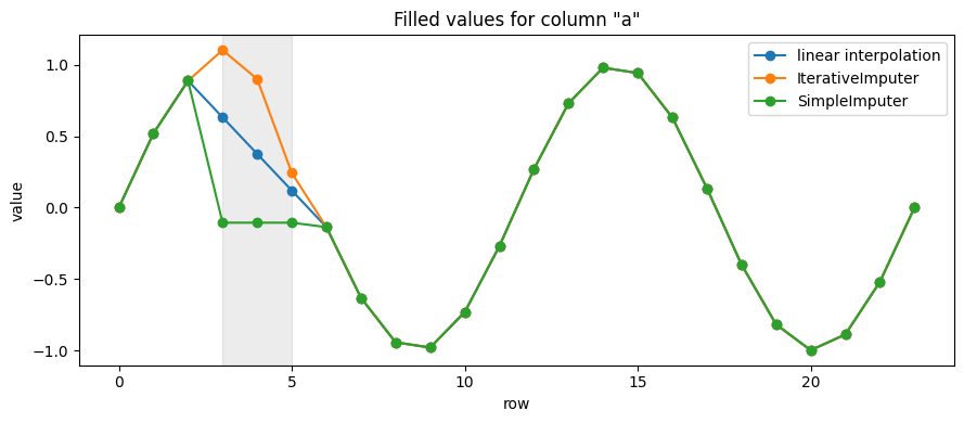
Interpolation uses each column’s own trend, while imputation models relationships across columns. Plotting the filled values for column a shows how the strategies differ where the data were missing (rows 3-5).
[5]:
missing_rows = [3, 4, 5]
comparison = pd.DataFrame({
    'linear interpolation': interpolated['a'],
    'IterativeImputer': iterative['a'],
    'SimpleImputer': simple['a'],
})
print('Values filled in for the missing rows of column "a":')
print(comparison.loc[missing_rows])

ax = comparison.plot(marker='o', figsize=(9, 4), title='Filled values for column "a"')
ax.axvspan(missing_rows[0], missing_rows[-1], alpha=0.15, color='gray')
ax.set_xlabel('row')
ax.set_ylabel('value')
plt.tight_layout()
plt.show()
Values filled in for the missing rows of column "a":
   linear interpolation  IterativeImputer  SimpleImputer
3              0.631872          1.102661      -0.105383
4              0.375859          0.899463      -0.105383
5              0.119846          0.243019      -0.105383