Data wrangling basics: supported filetypes

import datawrangler as dw
import numpy as np
import os
import pandas as pd
from matplotlib import pyplot as plt
from tutorial_helpers import data_file, image_file, text_file

Let’s load in some sample data:

dataframe = dw.io.load(data_file, index_col=0)
array = dataframe.values
image = dw.io.load(image_file)
text = dw.io.load(text_file)

Sample DataFrame:

dataframe

	FirstDim	SecondDim	ThirdDim	FourthDim	FifthDim
ByTwos
0	1	2	3	4	5
2	2	4	6	8	10
4	3	6	9	12	15
5	4	8	12	16	20
6	5	10	15	20	25
8	6	12	18	24	30
10	7	14	21	28	35

Sample Array

array

array([[ 1,  2,  3,  4,  5],
       [ 2,  4,  6,  8, 10],
       [ 3,  6,  9, 12, 15],
       [ 4,  8, 12, 16, 20],
       [ 5, 10, 15, 20, 25],
       [ 6, 12, 18, 24, 30],
       [ 7, 14, 21, 28, 35]])

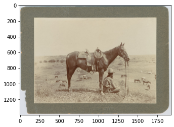
Sample image:

plt.imshow(image)

<matplotlib.image.AxesImage at 0x118e653c0>

Sample text:

print(text)

O give me a home where the buffaloes roam
Where the deer and the antelope play
Where seldom is heard a discouraging word
And the skies are not cloudy all day
Home, home on the range
Where the deer and the antelope play
Where seldom is heard a discouraging word
And the skies are not cloudy all day
Where the air is so pure and the zephyrs so free
And the breezes so balmy and light
That I would not exchange my home on the range
For all of the cities so bright
Home, home on the range
Where the deer and the antelope play
Where seldom is heard a discouraging word
And the skies are not cloudy all day
How often at night when the heavens are bright
With the light of the glittering stars
I stand there amazed and I ask as I gaze
Does their glory exceed that of ours?
Home, home on the range
Where the deer and the antelope play
Where seldom is heard a discouraging word
And the skies are not cloudy all day

Wrangling DataFrames

Wrangling a well-formed DataFrame just returns itself:

High-Performance DataFrames with Polars

data-wrangler now supports Polars, a lightning-fast DataFrame library that can provide 2-100x performance improvements over pandas for many operations. You can choose your DataFrame backend on a per-operation basis or globally.

Installation

Polars is now included as a core dependency of data-wrangler, so no additional installation is required!

Basic Polars Usage

You can specify the backend for any wrangling operation:

wrangled_df = dw.wrangle(dataframe)
assert np.allclose(dataframe, wrangled_df)
wrangled_df

	FirstDim	SecondDim	ThirdDim	FourthDim	FifthDim
ByTwos
0	1	2	3	4	5
2	2	4	6	8	10
4	3	6	9	12	15
5	4	8	12	16	20
6	5	10	15	20	25
8	6	12	18	24	30
10	7	14	21	28	35

Wrangling Arrays

Wrangling an Array turns it into a DataFrame. If the Array is 2D, the resulting DataFrame will have the same shape:

wrangled_array = dw.wrangle(array)
assert np.allclose(dataframe, wrangled_array)
wrangled_array

	0	1	2	3	4
0	1	2	3	4	5
1	2	4	6	8	10
2	3	6	9	12	15
3	4	8	12	16	20
4	5	10	15	20	25
5	6	12	18	24	30
6	7	14	21	28	35

Note that we’ve recovered the original DataFrame, but the index and column labels have been reset. We can provide these labels to the wrangle function. The array_kwargs keyword argument specifies how array (or array-like) data objects should be turned into DataFrames:

array_kwargs = {'index': dataframe.index, 'columns': dataframe.columns}
wrangled_array2 = dw.wrangle(array, array_kwargs=array_kwargs)
wrangled_array2

	FirstDim	SecondDim	ThirdDim	FourthDim	FifthDim
ByTwos
0	1	2	3	4	5
2	2	4	6	8	10
4	3	6	9	12	15
5	4	8	12	16	20
6	5	10	15	20	25
8	6	12	18	24	30
10	7	14	21	28	35

Loading data types from saved files

Every example above wrangled an in-memory Python object. data-wrangler can also wrangle data straight from a file on disk (or a URL): it auto-detects the format from the file extension, loads it, and wrangles the result in a single step. Here we round-trip the same DataFrame and Array through disk.

import tempfile

save_dir = tempfile.mkdtemp()

# --- DataFrame from a saved CSV file ---
csv_path = os.path.join(save_dir, 'sample.csv')
dataframe.to_csv(csv_path)
df_from_file = dw.wrangle(csv_path)   # pass the *path*; the CSV is loaded and wrangled automatically
print(f'Wrangled a {type(df_from_file).__name__} of shape {df_from_file.shape} from {os.path.basename(csv_path)}')
df_from_file.head()

Wrangled a DataFrame of shape (7, 6) from sample.csv

	ByTwos	FirstDim	SecondDim	ThirdDim	FourthDim	FifthDim
0	0	1	2	3	4	5
1	2	2	4	6	8	10
2	4	3	6	9	12	15
3	5	4	8	12	16	20
4	6	5	10	15	20	25

# --- Array from a saved .npy file ---
npy_path = os.path.join(save_dir, 'sample.npy')
np.save(npy_path, array)
array_from_file = dw.wrangle(npy_path)   # a NumPy file becomes a DataFrame
assert np.allclose(array_from_file, dataframe)
print(f'Wrangled a {type(array_from_file).__name__} of shape {array_from_file.shape} from {os.path.basename(npy_path)}')
array_from_file

Wrangled a DataFrame of shape (7, 5) from sample.npy

	0	1	2	3	4
0	1	2	3	4	5
1	2	4	6	8	10
2	3	6	9	12	15
3	4	8	12	16	20
4	5	10	15	20	25
5	6	12	18	24	30
6	7	14	21	28	35

Wrangling text data using natural language processing models

Next, let’s play with some text data. By default, data-wrangler embeds text using a Latent Dirichlet Allocation model trained on a curated version of Wikipedia, called the “minipedia” corpus. First we’ll split the text into its component lines, and then we’ll wrangle the result:

lines = text.split('\n')  # creates a list of strings (one string per line)
wrangled_text = dw.wrangle(lines)
wrangled_text

/Users/jmanning/.pyenv/versions/3.10.12/lib/python3.10/site-packages/tqdm/auto.py:21: TqdmWarning: IProgress not found. Please update jupyter and ipywidgets. See https://ipywidgets.readthedocs.io/en/stable/user_install.html
  from .autonotebook import tqdm as notebook_tqdm

loading corpus: minipedia...done!

	0	1	2	3	4	5	6	7	8	9	...	40	41	42	43	44	45	46	47	48	49
0	0.02	0.02	0.02	0.02	0.02	0.02	0.02	0.02	0.02	0.02	...	0.02	0.02	0.02	0.02	0.02	0.02	0.02	0.02	0.02	0.02
1	0.01	0.01	0.01	0.01	0.01	0.01	0.01	0.01	0.01	0.01	...	0.01	0.01	0.01	0.51	0.01	0.01	0.01	0.01	0.01	0.01
2	0.02	0.02	0.02	0.02	0.02	0.02	0.02	0.02	0.02	0.02	...	0.02	0.02	0.02	0.02	0.02	0.02	0.02	0.02	0.02	0.02
3	0.02	0.02	0.02	0.02	0.02	0.02	0.02	0.02	0.02	0.02	...	0.02	0.02	0.02	0.02	0.02	0.02	0.02	0.02	0.02	0.02
4	0.02	0.02	0.02	0.02	0.02	0.02	0.02	0.02	0.02	0.02	...	0.02	0.02	0.02	0.02	0.02	0.02	0.02	0.02	0.02	0.02
5	0.01	0.01	0.01	0.01	0.01	0.01	0.01	0.01	0.01	0.01	...	0.01	0.01	0.01	0.51	0.01	0.01	0.01	0.01	0.01	0.01
6	0.02	0.02	0.02	0.02	0.02	0.02	0.02	0.02	0.02	0.02	...	0.02	0.02	0.02	0.02	0.02	0.02	0.02	0.02	0.02	0.02
7	0.02	0.02	0.02	0.02	0.02	0.02	0.02	0.02	0.02	0.02	...	0.02	0.02	0.02	0.02	0.02	0.02	0.02	0.02	0.02	0.02
8	0.01	0.01	0.01	0.01	0.01	0.01	0.01	0.01	0.01	0.01	...	0.01	0.01	0.01	0.01	0.01	0.01	0.01	0.01	0.01	0.01
9	0.02	0.02	0.02	0.02	0.02	0.02	0.02	0.02	0.02	0.02	...	0.02	0.02	0.02	0.02	0.02	0.02	0.02	0.02	0.02	0.02
10	0.01	0.01	0.01	0.01	0.01	0.01	0.01	0.01	0.01	0.01	...	0.01	0.01	0.01	0.01	0.01	0.01	0.01	0.01	0.01	0.01
11	0.01	0.01	0.01	0.01	0.01	0.01	0.01	0.01	0.51	0.01	...	0.01	0.01	0.01	0.01	0.01	0.01	0.01	0.01	0.01	0.01
12	0.02	0.02	0.02	0.02	0.02	0.02	0.02	0.02	0.02	0.02	...	0.02	0.02	0.02	0.02	0.02	0.02	0.02	0.02	0.02	0.02
13	0.01	0.01	0.01	0.01	0.01	0.01	0.01	0.01	0.01	0.01	...	0.01	0.01	0.01	0.51	0.01	0.01	0.01	0.01	0.01	0.01
14	0.02	0.02	0.02	0.02	0.02	0.02	0.02	0.02	0.02	0.02	...	0.02	0.02	0.02	0.02	0.02	0.02	0.02	0.02	0.02	0.02
15	0.02	0.02	0.02	0.02	0.02	0.02	0.02	0.02	0.02	0.02	...	0.02	0.02	0.02	0.02	0.02	0.02	0.02	0.02	0.02	0.02
16	0.01	0.01	0.01	0.01	0.01	0.01	0.01	0.01	0.01	0.01	...	0.01	0.01	0.01	0.01	0.01	0.51	0.01	0.01	0.01	0.01
17	0.02	0.02	0.02	0.02	0.02	0.02	0.02	0.02	0.02	0.02	...	0.02	0.02	0.02	0.02	0.02	0.02	0.02	0.02	0.02	0.02
18	0.01	0.01	0.01	0.01	0.01	0.01	0.01	0.01	0.01	0.01	...	0.01	0.01	0.01	0.01	0.01	0.01	0.01	0.01	0.01	0.01
19	0.02	0.02	0.02	0.02	0.02	0.02	0.02	0.02	0.02	0.02	...	0.02	0.02	0.02	0.02	0.02	0.02	0.02	0.02	0.02	0.02
20	0.02	0.02	0.02	0.02	0.02	0.02	0.02	0.02	0.02	0.02	...	0.02	0.02	0.02	0.02	0.02	0.02	0.02	0.02	0.02	0.02
21	0.01	0.01	0.01	0.01	0.01	0.01	0.01	0.01	0.01	0.01	...	0.01	0.01	0.01	0.51	0.01	0.01	0.01	0.01	0.01	0.01
22	0.02	0.02	0.02	0.02	0.02	0.02	0.02	0.02	0.02	0.02	...	0.02	0.02	0.02	0.02	0.02	0.02	0.02	0.02	0.02	0.02
23	0.02	0.02	0.02	0.02	0.02	0.02	0.02	0.02	0.02	0.02	...	0.02	0.02	0.02	0.02	0.02	0.02	0.02	0.02	0.02	0.02

24 rows × 50 columns

In the resulting DataFrame, each row corresponds to a line of text, and each column corresponds to an embedding dimension. To get a better feel for what these dimensions mean, we can use the return_model flag to get back the fitted model, and then we can examine the top-weighted words from each topic:

wrangled_text2, text_model = dw.wrangle(lines, text_kwargs={'return_model': True})

# display top words from the model
def get_top_words(model, n_words=10):
  vectorizer = model[0]['model']
  embedder = model[1]['model']

  vocab = {v: k for k, v in vectorizer.vocabulary_.items()}
  top_words = []
  for k in range(embedder.components_.shape[0]):
      top_words.append([vocab[i] for i in np.argsort(embedder.components_[k, :])[::-1][:n_words]])
  return top_words

def display_top_words(model, n_words=10):
  for k, w in enumerate(get_top_words(model, n_words=n_words)):
      print(f'Topic {k}: {", ".join(w)}')

print(f'Top words from each of the {wrangled_text2.shape[1]} discovered topics:\n')
display_top_words(text_model)

Top words from each of the 50 discovered topics:

Topic 0: cells, cell, blood, structures, skin, growth, layer, functions, outer, internal
Topic 1: sea, ice, land, river, ft, winter, weather, rock, climate, flow
Topic 2: music, sound, rock, play, played, classical, style, plays, note, double
Topic 3: elements, element, table, earth, classical, symbol, matter, names, things, theory
Topic 4: face, tools, tool, die, edge, foundation, stone, removed, base, skin
Topic 5: building, built, house, buildings, floor, wall, room, construction, walls, houses
Topic 6: species, fish, wild, male, female, live, young, feed, adult, humans
Topic 7: population, african, cultural, cultures, africa, native, al, regions, region, asian
Topic 8: soil, plants, plant, root, matter, growth, brown, field, dry, formation
Topic 9: women, sexual, men, female, male, woman, mother, man, child, birth
Topic 10: game, play, team, played, rules, sports, field, events, competition, association
Topic 11: pressure, heat, temperature, glass, liquid, flow, hot, fluid, cold, volume
Topic 12: angle, points, lines, normal, numbers, units, equal, value, measure, distance
Topic 13: death, dead, remains, die, carried, performed, medical, removed, blood, circumstances
Topic 14: store, storage, distribution, items, goods, space, stored, department, big, equipment
Topic 15: project, performance, computer, techniques, construction, patterns, technology, site, style, machine
Topic 16: blood, disease, risk, health, treatment, heart, diseases, skin, causes, medical
Topic 17: political, theory, science, concept, definition, property, economic, cultural, scientific, knowledge
Topic 18: chain, title, medicine, medical, equivalent, review, degree, usage, college, post
Topic 19: foot, feet, running, height, figure, figures, step, cm, fall, standing
Topic 20: animals, animal, humans, ago, living, evolution, species, million, plants, evolved
Topic 21: speed, electric, electrical, frequency, devices, mechanical, device, machine, sound, motion
Topic 22: color, yellow, colors, blue, eye, skin, dark, green, visible, brown
Topic 23: green, blue, party, political, yellow, dark, spring, brown, feature, environmental
Topic 24: military, forces, force, charge, service, units, field, operations, unit, mounted
Topic 25: million, 2008, 2011, 2007, 2010, 2009, 2012, 2013, 2006, march
Topic 26: health, service, services, care, medical, poor, community, hours, treatment, access
Topic 27: training, degree, professional, science, degrees, field, education, programs, engineering, knowledge
Topic 28: church, god, christian, religious, roman, tradition, religion, man, story, traditions
Topic 29: earth, wind, sun, scale, mass, energy, core, space, objects, night
Topic 30: class, japanese, ii, saw, japan, russian, germany, france, anti, britain
Topic 31: city, street, cities, town, urban, london, department, road, paris, center
Topic 32: wood, head, metal, mm, steel, plastic, cut, flat, diameter, shaped
Topic 33: language, languages, key, writing, words, data, test, numbers, computer, formal
Topic 34: film, television, image, video, record, records, released, images, character, media
Topic 35: art, objects, object, museum, glass, collection, works, subject, fine, gallery
Topic 36: paper, books, money, online, exchange, published, issued, text, value, electronic
Topic 37: 40, class, operation, australian, 27, buildings, property, 1970s, properties, cities
Topic 38: energy, gas, oil, carbon, chemical, compounds, acid, reaction, properties, liquid
Topic 39: record, head, nations, government, service, class, operate, represent, past, formal
Topic 40: worn, wear, cross, clothing, fashion, style, men, women, styles, popularity
Topic 41: children, school, education, child, schools, college, young, secondary, families, care
Topic 42: fruit, leaves, tree, trees, plant, varieties, grown, plants, species, served
Topic 43: legal, court, government, rights, civil, property, laws, service, federal, serve
Topic 44: management, organization, business, board, organizations, company, security, companies, activities, course
Topic 45: india, bc, king, chinese, roman, east, royal, empire, indian, spanish
Topic 46: self, behavior, theory, experience, individuals, relationship, studies, positive, negative, activity
Topic 47: market, products, product, price, supply, industry, trade, sold, demand, goods
Topic 48: vehicles, road, built, safety, transport, speed, electric, model, double, models
Topic 49: gold, iron, silver, metal, steel, bc, value, stone, carbon, pure

Then we can ask which topics had the most weight in each line:

i = 1
line_embedding = wrangled_text2.loc[i].values
line_top_topic = np.where(line_embedding == np.max(line_embedding))[0][0]

print(f'Line {i} put the most weight on topic {line_top_topic}: {lines[i]}')

Line 1 put the most weight on topic 10: Where the deer and the antelope play

Note that each time the model is re-trained, the topic weights will change. If all text data are wrangled in a single pass, data-wrangler will automatically apply the same model to all text data. However, if the data are wrangled in multiple calls to dw.wrangle, the model fit during the first pass should be re-used in subsequent analyses:

def match(a, b, type):
    if np.allclose(a, b):
        print(f'{type.capitalize()}s match!')
    else:
        print(f'{type.capitalize()}s do NOT match!')

match(wrangled_text, wrangled_text2, 'topic')

Topics do NOT match!

We can re-apply the already-fitted model to “new” text:

wrangled_text3 = dw.wrangle(lines, text_kwargs={'model': text_model})
match(wrangled_text2, wrangled_text3, 'topic')

Topics do NOT match!

Modern Text Processing with Sentence-Transformers

In addition to scikit-learn text embedding models, data-wrangler provides comprehensive support for state-of-the-art sentence-transformers models via HuggingFace.

Installation Requirements

Sentence-transformers support requires additional ML libraries. To keep data-wrangler lightweight, these are optional dependencies:

pip install --upgrade "pydata-wrangler[hf]"

This installs sentence-transformers, transformers, and related HuggingFace libraries.

Popular Sentence-Transformers Models

Different models are optimized for different tasks:

• ``all-MiniLM-L6-v2``: Fast, general-purpose sentence embeddings (384 dimensions)

• ``all-mpnet-base-v2``: High-quality sentence embeddings (768 dimensions)

• ``paraphrase-MiniLM-L6-v2``: Optimized for paraphrase detection

• ``all-distilroberta-v1``: Balanced performance and speed

Basic Usage

Here’s how to use sentence-transformers with your text data:

# High-quality model - better for production applications
# Using simplified API - just pass the model name as a string!
quality_embeddings = dw.wrangle(lines, text_kwargs={'model': 'all-mpnet-base-v2'})

print(f"Quality model embeddings shape: {quality_embeddings.shape}")
print(f"Quality model (first few dimensions):")
quality_embeddings.iloc[:3, :5]

Warning: You are sending unauthenticated requests to the HF Hub. Please set a HF_TOKEN to enable higher rate limits and faster downloads.
Loading weights: 100%|██████████| 199/199 [00:00<00:00, 7226.05it/s]

Quality model embeddings shape: (24, 768)
Quality model (first few dimensions):

	0	1	2	3	4
0	-0.012806	0.115035	-0.002113	-0.020551	0.013699
1	0.014780	-0.007010	-0.022478	0.015275	-0.052132
2	0.025268	0.023997	0.028487	-0.006982	0.029362

Model Comparison

Notice the difference in embedding dimensions:

• Fast model (all-MiniLM-L6-v2): 384 dimensions - good for speed and memory efficiency

• Quality model (all-mpnet-base-v2): 768 dimensions - better semantic understanding

Practical Applications

Different models work better for different tasks:

1. Similarity Search: Use all-MiniLM-L6-v2 for fast similarity search

2. Semantic Analysis: Use all-mpnet-base-v2 for deeper semantic understanding

3. Paraphrase Detection: Use paraphrase-MiniLM-L6-v2 for finding similar content

Let’s see how these embeddings can be used for similarity analysis:

# Fast model - good for quick prototyping
# Using simplified API - just pass the model name as a string!
fast_embeddings = dw.wrangle(lines, text_kwargs={'model': 'all-MiniLM-L6-v2'})

print(f"Fast model embeddings shape: {fast_embeddings.shape}")
print(f"Fast model (first few dimensions):")
fast_embeddings.iloc[:3, :5]

# `sentence_embeddings` is an alias used later when comparing batched vs. separate wrangling
sentence_embeddings = fast_embeddings

Loading weights: 100%|██████████| 103/103 [00:00<00:00, 8563.37it/s]

Fast model embeddings shape: (24, 384)
Fast model (first few dimensions):

# Example: Find similar lines using cosine similarity
from sklearn.metrics.pairwise import cosine_similarity
import numpy as np

# Calculate similarity matrix
similarity_matrix = cosine_similarity(fast_embeddings)

# Find the most similar lines to the first line
line_0_similarities = similarity_matrix[0]
most_similar_indices = np.argsort(line_0_similarities)[-3:]  # Top 3 similar lines

print("Original line 0:", lines[0])
print("\nMost similar lines:")
for idx in reversed(most_similar_indices):
    if idx != 0:  # Don't include the line itself
        print(f"Line {idx} (similarity: {line_0_similarities[idx]:.3f}): {lines[idx]}")

Original line 0: O give me a home where the buffaloes roam

Most similar lines:
Line 20 (similarity: 0.405): Home, home on the range
Line 12 (similarity: 0.405): Home, home on the range

Scikit-learn text models: different models and different corpora

The default text pipeline (CountVectorizer then LatentDirichletAllocation) is only one option. Any scikit-learn text vectorizer or decomposition/topic model may be used, and each is trained on a corpus that you choose with the corpus keyword. data-wrangler ships several small, pre-cached corpora ('minipedia', 'sotus', 'neurips', 'khan'). Below we embed the same lines with a few different models, trained on two different built-in corpora.

# The same text, embedded with different sklearn pipelines trained on different corpora
sklearn_examples = {
    'CountVectorizer (minipedia)': {'model': 'CountVectorizer', 'corpus': 'minipedia'},
    'Count -> LDA topics (minipedia)': {'model': ['CountVectorizer', 'LatentDirichletAllocation'], 'corpus': 'minipedia'},
    'Count -> LDA topics (sotus)': {'model': ['CountVectorizer', 'LatentDirichletAllocation'], 'corpus': 'sotus'},
    'Tfidf -> TruncatedSVD (sotus)': {'model': ['TfidfVectorizer', 'TruncatedSVD'], 'corpus': 'sotus'},
}

for name, kw in sklearn_examples.items():
    embedded = dw.wrangle(lines, text_kwargs=kw)
    print(f'{name:34s} -> {embedded.shape[0]} rows x {embedded.shape[1]} features')

CountVectorizer (minipedia)        -> 24 rows x 1220 features
Count -> LDA topics (minipedia)    -> 24 rows x 50 features
loading corpus: sotus...done!Count -> LDA topics (sotus)        -> 24 rows x 50 features
Tfidf -> TruncatedSVD (sotus)      -> 24 rows x 29 features

Vectorization vs. embedding

There are two fundamentally different ways data-wrangler turns text into numbers:

• Vectorization (scikit-learn, e.g. CountVectorizer): the model is trained on your corpus to build a vocabulary, then each document becomes a sparse vector of word counts (or TF-IDF weights). The number of columns equals the vocabulary size, and the values are interpretable (counts of specific words).

• Embedding with an already-trained model (sentence-transformers, e.g. all-MiniLM-L6-v2): the model is pre-trained on massive external data, so it needs no corpus. Each document becomes a compact, dense vector that captures meaning, so semantically similar sentences land near each other.

sample = ['I love my dog', 'My puppy is adorable', 'The stock market fell today']

# Vectorization: CountVectorizer trained on a corpus -> sparse word counts
counts = dw.wrangle(sample, text_kwargs={'model': 'CountVectorizer', 'corpus': 'minipedia'})

# Embedding: a pre-trained sentence-transformer applied directly (no corpus needed)
embeddings = dw.wrangle(sample, text_kwargs={'model': 'all-MiniLM-L6-v2'})

from sklearn.metrics.pairwise import cosine_similarity
print(f'CountVectorizer    -> {counts.shape[1]} columns (vocabulary), mostly zeros')
print(f'Sentence embedding -> {embeddings.shape[1]} dense columns (meaning)')
print()
print('Semantic similarity (the two dog sentences should be far more similar than dog vs. stocks):')
sim = cosine_similarity(embeddings)
print(f'  dog / puppy  similarity: {sim[0, 1]:.3f}')
print(f'  dog / stocks similarity: {sim[0, 2]:.3f}')

Loading weights: 100%|██████████| 103/103 [00:00<00:00, 16031.37it/s]

CountVectorizer    -> 1220 columns (vocabulary), mostly zeros
Sentence embedding -> 384 dense columns (meaning)

Semantic similarity (the two dog sentences should be far more similar than dog vs. stocks):
  dog / puppy  similarity: 0.641
  dog / stocks similarity: 0.022

Training on a Hugging-Face corpus

Beyond the built-in corpora, corpus accepts any Hugging-Face dataset, referenced by its full namespace/name id (bare legacy names are rejected by datasets >= 4). Use the config keyword to pick a dataset variant. Here we train a topic model on the Children’s Book Test corpus ('cam-cst/cbt', config 'raw'):

cbt_topics = dw.wrangle(lines, text_kwargs={'model': ['CountVectorizer', 'LatentDirichletAllocation'],
                                            'corpus': 'cam-cst/cbt', 'config': 'raw'})
print(f'Topic embedding trained on cam-cst/cbt: {cbt_topics.shape[0]} rows x {cbt_topics.shape[1]} topics')
cbt_topics.head()

Topic embedding trained on cam-cst/cbt: 24 rows x 50 topics

	0	1	2	3	4	5	6	7	8	9	...	40	41	42	43	44	45	46	47	48	49
0	0.010000	0.010000	0.010000	0.010000	0.010000	0.010000	0.010000	0.010000	0.010000	0.010000	...	0.010000	0.010000	0.010000	0.510000	0.010000	0.010000	0.010000	0.010000	0.010000	0.010000
1	0.020000	0.020000	0.020000	0.020000	0.020000	0.020000	0.020000	0.020000	0.020000	0.020000	...	0.020000	0.020000	0.020000	0.020000	0.020000	0.020000	0.020000	0.020000	0.020000	0.020000
2	0.020000	0.020000	0.020000	0.020000	0.020000	0.020000	0.020000	0.020000	0.020000	0.020000	...	0.020000	0.020000	0.020000	0.020000	0.020000	0.020000	0.020000	0.020000	0.020000	0.020000
3	0.006667	0.006667	0.006667	0.006667	0.006667	0.006667	0.006667	0.006667	0.006667	0.006667	...	0.006667	0.006667	0.006667	0.006667	0.006667	0.006667	0.006667	0.006667	0.006667	0.006667
4	0.010000	0.010000	0.010000	0.010000	0.010000	0.010000	0.010000	0.010000	0.010000	0.510000	...	0.010000	0.010000	0.010000	0.010000	0.010000	0.010000	0.010000	0.010000	0.010000	0.010000

5 rows × 50 columns

Wrangling images

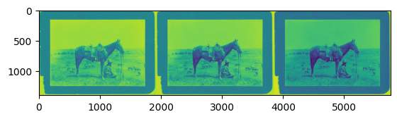
Images (stored in any format supported by matplotlib) treated as Arrays. Images are wrangled into DataFrames by slicing the image along axis 2 (i.e., the color dimension), horizontally concatenating the slices, and then turning the result into a DataFrame. In general, this approach is taken for all high-dimensional (> 2D) Arrays:

wrangled_image = dw.wrangle(image)
plt.imshow(wrangled_image);

Objects, file paths, and URLs

Data supplied to data-wrangler may be passed in directly as a Python object that is already loaded into memory (as in the above examples). However, data may also be supplied as a (string) file path or URL. For example, wrangling the already loaded-in image versus wrangling the image’s file path will yield the same result:

wrangled_image_from_path = dw.wrangle(image_file)
match(wrangled_image, wrangled_image_from_path, 'image')

Images match!

Handling multiple data types

Multiple objects, file paths, or URLs may be wrangled in a single function call. If desired, type-specific wrangling preferences may be provided. Specifying return_dtype=True also returns a list of the automatically detected data types for each object:

# Using simplified API - just pass the model name as a string\!
text_kwargs = {'model': 'all-MiniLM-L6-v2'}

i = 10
first_lines = lines[:i]
last_lines = lines[i:]

wrangled_data, dtypes = dw.wrangle([dataframe, array, image_file, first_lines, last_lines],
                                   text_kwargs=text_kwargs,
                                   return_dtype=True)

Loading weights: 100%|██████████| 103/103 [00:00<00:00, 13232.46it/s]
Loading weights: 100%|██████████| 103/103 [00:00<00:00, 14084.48it/s]

We can check the inferred datatypes:

dtypes

['dataframe', 'array', 'array', 'text', 'text']

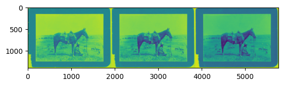
We can also verify that when the data are wrangled simultaneously, we get the same results as when each object is wrangled separately. For example, here’s the newly wrangled image:

# visualize the wrangled image
plt.imshow(wrangled_data[2])

<matplotlib.image.AxesImage at 0x13b4fb7c0>

And here’s how the text embeddings compare to our previous results:

# compare the first lines' embeddings:
match(sentence_embeddings.iloc[:i], wrangled_data[3], 'first lines\'s sentence-transformers embedding')

# compare the last lines' embeddings
match(sentence_embeddings.iloc[i:], wrangled_data[4], 'last lines\'s sentence-transformers embedding')

First lines's sentence-transformers embeddings match!
Last lines's sentence-transformers embeddings match!

Check out the other tutorials for more advanced data wrangling functions!

# Wrangle data using Polars backend for high performance
import polars as pl

# Convert array to Polars DataFrame
polars_df = dw.wrangle(array, backend='polars')
print(f"Polars DataFrame type: {type(polars_df)}")
print(f"Shape: {polars_df.shape}")
polars_df.head()

Polars DataFrame type: <class 'polars.dataframe.frame.DataFrame'>
Shape: (7, 5)

shape: (5, 5)

0	1	2	3	4
i64	i64	i64	i64	i64
1	2	3	4	5
2	4	6	8	10
3	6	9	12	15
4	8	12	16	20
5	10	15	20	25

Cross-Backend Conversion

You can convert between pandas and Polars DataFrames seamlessly:

# Convert pandas DataFrame to Polars
pandas_df = wrangled_df  # Our original pandas DataFrame
polars_from_pandas = dw.wrangle(pandas_df, backend='polars')

print(f"Original: {type(pandas_df)}")
print(f"Converted to Polars: {type(polars_from_pandas)}")

# Convert Polars DataFrame back to pandas
pandas_from_polars = dw.wrangle(polars_from_pandas, backend='pandas')
print(f"Converted back to pandas: {type(pandas_from_polars)}")

# Verify data is preserved
import numpy as np
print(f"Data preserved: {np.allclose(pandas_df.values, pandas_from_polars.values)}")

Original: <class 'pandas.core.frame.DataFrame'>
Converted to Polars: <class 'polars.dataframe.frame.DataFrame'>
Converted back to pandas: <class 'pandas.core.frame.DataFrame'>
Data preserved: True

Global Backend Configuration

You can set a global preference for DataFrame backend:

# Configure global backend preference
from datawrangler.core.configurator import set_dataframe_backend, get_dataframe_backend

# Check current default
print(f"Current default backend: {get_dataframe_backend()}")

# Set global preference to Polars
set_dataframe_backend('polars')
print(f"New default backend: {get_dataframe_backend()}")

# Now all operations use Polars by default
global_polars_df = dw.wrangle(array)  # No need to specify backend='polars'
print(f"Global setting result: {type(global_polars_df)}")

# Reset to pandas for rest of tutorial
set_dataframe_backend('pandas')
print(f"Reset to: {get_dataframe_backend()}")

Current default backend: pandas
New default backend: polars
Global setting result: <class 'pandas.core.frame.DataFrame'>
Reset to: pandas

Text Processing with Polars

Text processing also supports the Polars backend for high-performance embeddings:

# Text embeddings with Polars backend for better performance
sample_texts = ["Machine learning is fascinating",
                "Data science combines statistics and programming",
                "Polars is a fast DataFrame library"]

# Process text with Polars backend
polars_text_df = dw.wrangle(sample_texts, backend='polars')
print(f"Text embeddings with Polars: {type(polars_text_df)}")
print(f"Shape: {polars_text_df.shape}")

# Compare with pandas backend
pandas_text_df = dw.wrangle(sample_texts, backend='pandas')
print(f"Text embeddings with pandas: {type(pandas_text_df)}")
print(f"Shape: {pandas_text_df.shape}")

# Both should have the same shape
print(f"Same embedding dimensions: {polars_text_df.shape == pandas_text_df.shape}")

Text embeddings with Polars: <class 'polars.dataframe.frame.DataFrame'>
Shape: (3, 50)
Text embeddings with pandas: <class 'pandas.core.frame.DataFrame'>
Shape: (3, 50)
Same embedding dimensions: True

Performance Benefits

Polars offers significant performance advantages, especially for:

• Large datasets: 2-10x faster operations on datasets with millions of rows

• Aggregations: Group-by operations and statistical computations

• Memory efficiency: Lower memory usage with columnar data format

• Parallel processing: Built-in parallelization for multi-core systems

The choice between pandas and Polars depends on your specific needs:

• Use pandas for: Familiarity, ecosystem compatibility, complex transformations

• Use Polars for: Performance, large datasets, memory efficiency, parallel processing

Automatic Type Preservation

data-wrangler automatically preserves your DataFrame type when no backend is specified:

Performance Benchmark Example

Here’s a practical example showing the performance difference between pandas and Polars for array conversion:

# Demonstrate automatic type preservation
import pandas as pd
import polars as pl

# Create DataFrames of each type
pandas_input = pd.DataFrame({'A': [1, 2, 3], 'B': [4, 5, 6]})
polars_input = pl.DataFrame({'A': [1, 2, 3], 'B': [4, 5, 6]})

# Wrangle without specifying backend - type is preserved
pandas_output = dw.wrangle(pandas_input)
polars_output = dw.wrangle(polars_input)

print(f"Pandas input: {type(pandas_input)} -> Output: {type(pandas_output)}")
print(f"Polars input: {type(polars_input)} -> Output: {type(polars_output)}")
print("✅ Types automatically preserved!")

Pandas input: <class 'pandas.core.frame.DataFrame'> -> Output: <class 'pandas.core.frame.DataFrame'>
Polars input: <class 'polars.dataframe.frame.DataFrame'> -> Output: <class 'polars.dataframe.frame.DataFrame'>
✅ Types automatically preserved!

import time
import numpy as np

# Create a moderately sized array for benchmarking
large_array = np.random.rand(10000, 50)
print(f"Array shape: {large_array.shape}")

# Benchmark pandas backend
start_time = time.time()
pandas_result = dw.wrangle(large_array, backend='pandas')
pandas_time = time.time() - start_time

# Benchmark Polars backend
start_time = time.time()
polars_result = dw.wrangle(large_array, backend='polars')
polars_time = time.time() - start_time

print(f"\n📊 Performance Comparison:")
print(f"Pandas backend: {pandas_time:.4f} seconds")
print(f"Polars backend: {polars_time:.4f} seconds")
print(f"Speedup: {pandas_time/polars_time:.1f}x faster with Polars")

# Verify results are equivalent
print(f"\n✅ Results equivalent: {np.allclose(pandas_result.values, polars_result.to_pandas().values)}")

Array shape: (10000, 50)

📊 Performance Comparison:
Pandas backend: 0.0003 seconds
Polars backend: 0.0009 seconds
Speedup: 0.4x faster with Polars

✅ Results equivalent: True

Summary: Choosing the Right Backend

data-wrangler now provides flexible DataFrame backend support:

Feature	pandas	Polars
Performance	Standard	2-100x faster
Memory Usage	Higher	Lower (columnar)
Ecosystem	Mature, extensive	Growing rapidly
Learning Curve	Familiar to most	Similar API
Best For	General use, prototyping	Large data, production

Quick Start Guide

# Basic usage - specify backend per operation
import datawrangler as dw

# Use pandas (default)
df_pandas = dw.wrangle(data)

# Use Polars for performance
df_polars = dw.wrangle(data, backend='polars')

# Set global preference
from datawrangler.core.configurator import set_dataframe_backend
set_dataframe_backend('polars')  # All operations use Polars

Both backends support all data-wrangler functionality including text processing, array conversion, and complex data wrangling pipelines. Choose the backend that best fits your performance requirements and workflow preferences!